

python

산업 제조
파이썬의 SciPy 수학, 과학, 공학 및 기술 문제를 해결하는 데 사용되는 오픈 소스 라이브러리입니다. 이를 통해 사용자는 광범위한 고급 Python 명령을 사용하여 데이터를 조작하고 데이터를 시각화할 수 있습니다. SciPy는 Python NumPy 확장을 기반으로 합니다. SciPy는 "Sigh Pi"로도 발음됩니다.
SciPy의 하위 패키지:
이 Python SciPy 자습서에서는 다음을 배우게 됩니다.
pip를 통해 Windows에 SciPy를 설치할 수도 있습니다.
Python3 -m pip install --user numpy scipy
Linux에 Scipy 설치
sudo apt-get install python-scipy python-numpy
Mac에 SciPy 설치
sudo port install py35-scipy py35-numpy
SciPy Python 학습을 시작하기 전에 기본 기능과 다양한 유형의 NumPy 배열을 알아야 합니다.
SciPy 모듈 및 Numpy를 가져오는 표준 방법:
from scipy import special   #same for other modules
import numpy as np
I/O 패키지인 Scipy에는 Matlab, Arff, Wave, Matrix Market, IDL, NetCDF, TXT, CSV 및 바이너리 형식과 같은 다양한 파일 형식으로 작업할 수 있는 광범위한 기능이 있습니다.
MatLab에서 정기적으로 사용되는 파일 형식 Python SciPy 예를 하나 들어보겠습니다.
 import numpy as np
 from scipy import io as sio
 array = np.ones((4, 4))
 sio.savemat('example.mat', {'ar': array})
 data = sio.loadmat(‘example.mat', struct_as_record=True)
 data['ar']
출력:
array([[ 1., 1., 1., 1.],
           [ 1., 1., 1., 1.],
           [ 1., 1., 1., 1.],
           [ 1., 1., 1., 1.]])
코드 설명
help(scipy.special)
Output :
NAME
    scipy.special

DESCRIPTION
    ========================================
    Special functions (:mod:`scipy.special`)
    ========================================

    .. module:: scipy.special

    Nearly all of the functions below are universal functions and follow
    broadcasting and automatic array-looping rules. Exceptions are noted.
입방근 함수는 값의 입방근을 찾습니다.
구문:
scipy.special.cbrt(x)
예:
from scipy.special import cbrt
#Find cubic root of 27 & 64 using cbrt() function
cb = cbrt([27, 64])
#print value of cb
print(cb)
출력: 배열([3., 4.])
지수 함수는 10**x 요소별로 계산합니다.
예:
from scipy.special import exp10
#define exp10 function and pass value in its
exp = exp10([1,10])
print(exp)
출력:[1.e+01 1.e+10]
SciPy는 순열 및 조합을 계산하는 기능도 제공합니다.
조합 – scipy.special.comb(N,k)
예:
from scipy.special import comb
#find combinations of 5, 2 values using comb(N, k)
com = comb(5, 2, exact = False, repetition=True)
print(com)
출력:15.0
순열 –
scipy.special.perm(N,k)
예:
from scipy.special import perm
#find permutation of 5, 2 using perm (N, k) function
per = perm(5, 2, exact = True)
print(per)
출력:20
Log Sum Exponential은 합계 지수 입력 요소의 로그를 계산합니다.
구문:
scipy.special.logsumexp(x)
N번째 정수 차수 계산 함수
구문:
scipy.special.jn()
이제 scipy.linalg로 몇 가지 테스트를 해보겠습니다.
행렬 계산 2차원 행렬의
from scipy import linalg
import numpy as np
#define square matrix
two_d_array = np.array([ [4,5], [3,2] ])
#pass values to det() function
linalg.det( two_d_array )
출력: -7.0
역행렬 –
scipy.linalg.inv()
Scipy의 역행렬은 모든 정방행렬의 역행렬을 계산합니다.
보자,
from scipy import linalg
import numpy as np
# define square matrix
two_d_array = np.array([ [4,5], [3,2] ])
#pass value to function inv()
linalg.inv( two_d_array )
출력:
array( [[-0.28571429,  0.71428571],
       [ 0.42857143, -0.57142857]] )
scipy.linalg.eig()
예
from scipy import linalg
import numpy as np
#define two dimensional array
arr = np.array([[5,4],[6,3]])
#pass value into function
eg_val, eg_vect = linalg.eig(arr)
#get eigenvalues
print(eg_val)
#get eigenvectors
print(eg_vect)
출력:
[ 9.+0.j -1.+0.j] #eigenvalues
 [ [ 0.70710678 -0.5547002 ] #eigenvectors
   [ 0.70710678  0.83205029] ]
예: Matplotlib 라이브러리를 사용하여 웨이브하고 보여줍니다. 우리는 sin(20 × 2πt)
의 간단한 주기 함수 예제를 취합니다.
%matplotlib inline
from matplotlib import pyplot as plt
import numpy as np

#Frequency in terms of Hertz
fre  = 5
#Sample rate
fre_samp = 50
t = np.linspace(0, 2, 2 * fre_samp, endpoint = False )
a = np.sin(fre  * 2 * np.pi * t)
figure, axis = plt.subplots()
axis.plot(t, a)
axis.set_xlabel ('Time (s)')
axis.set_ylabel ('Signal amplitude')
plt.show()
출력:
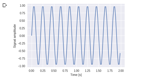
당신은 이것을 볼 수 있습니다. 주파수는 5Hz이고 신호는 1/5초 동안 반복됩니다. 특정 시간으로 호출됩니다.
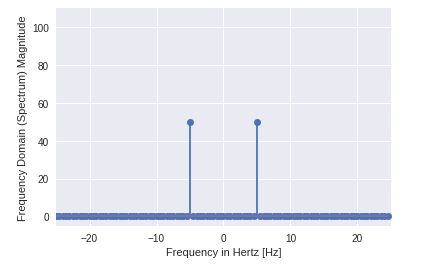
이제 DFT 응용 프로그램의 도움으로 이 정현파를 사용하겠습니다.
from scipy import fftpack

A = fftpack.fft(a)
frequency = fftpack.fftfreq(len(a)) * fre_samp
figure, axis = plt.subplots()

axis.stem(frequency, np.abs(A))
axis.set_xlabel('Frequency in Hz')
axis.set_ylabel('Frequency Spectrum Magnitude')
axis.set_xlim(-fre_samp / 2, fre_samp/ 2)
axis.set_ylim(-5, 110)
plt.show()
출력:
%matplotlib inline
import matplotlib.pyplot as plt
from scipy import optimize
import numpy as np
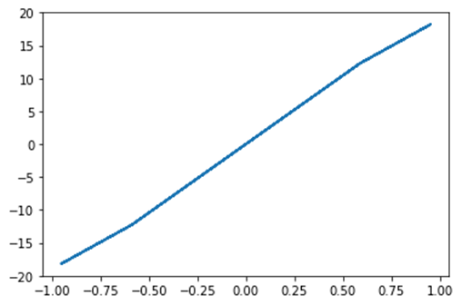
def function(a):
return a*2 + 20 * np.sin(a)
plt.plot(a, function(a))
plt.show()
#use BFGS algorithm for optimization
optimize.fmin_bfgs(function, 0)
출력:
최적화가 성공적으로 종료되었습니다.
현재 함수 값:-23.241676
반복:4
기능 평가:18
기울기 평가:6
배열([-1.67096375])
optimize.basinhopping(함수, 0)
출력:
fun: -23.241676238045315
 lowest_optimization_result:
      fun: -23.241676238045315
 hess_inv: array([[0.05023331]])
      jac: array([4.76837158e-07])
  message: 'Optimization terminated successfully.'
     nfev: 15
      nit: 3
     njev: 5
   status: 0
  success: True
        x: array([-1.67096375])
                    message: ['requested number of basinhopping iterations completed successfully']
      minimization_failures: 0
                       nfev: 1530
                        nit: 100
                       njev: 510
               x: array([-1.67096375])
import numpy as np
from scipy.optimize import minimize
#define function f(x)
def f(x):
    return .4*(1 - x[0])**2

optimize.minimize(f, [2, -1], method="Nelder-Mead")
출력:
final_simplex: (array([[ 1.        , -1.27109375],
       [ 1.        , -1.27118835],
       [ 1.        , -1.27113762]]), array([0., 0., 0.]))
           fun: 0.0
       message: 'Optimization terminated successfully.'
          nfev: 147
           nit: 69
        status: 0
       success: True
             x: array([ 1.        , -1.27109375])
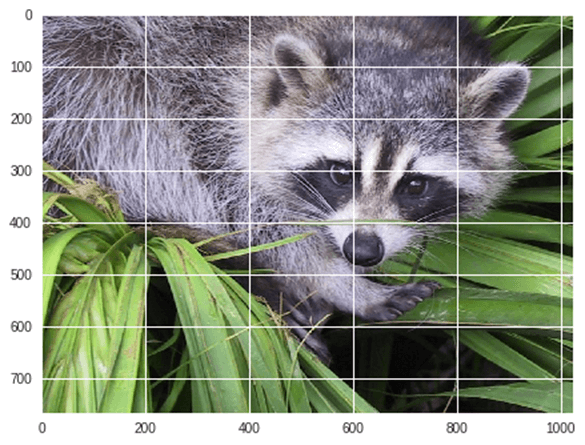
예: 이미지의 기하학적 변환을 예로 들어 보겠습니다.
from scipy import misc
from matplotlib import pyplot as plt
import numpy as np
#get face image of panda from misc package
panda = misc.face()
#plot or show image of face
plt.imshow( panda )
plt.show()
출력:

이제 뒤집기 현재 이미지:
#Flip Down using scipy misc.face image
flip_down = np.flipud(misc.face())
plt.imshow(flip_down)
plt.show()
출력:
예: Scipy를 사용한 이미지 회전,
from scipy import ndimage, misc
from matplotlib import pyplot as plt
panda = misc.face()
#rotatation function of scipy for image – image rotated 135 degree
panda_rotate = ndimage.rotate(panda, 135)
plt.imshow(panda_rotate)
plt.show()
출력:
예: 이제 단일 통합의 예를 들어보세요.

여기 a 상한선이고 b 하한
from scipy import integrate
# take f(x) function as f
f = lambda x : x**2
#single integration with a = 0 & b = 1
integration = integrate.quad(f, 0 , 1)
print(integration)
출력:
(0.33333333333333337, 3.700743415417189e-15)
여기서 함수는 첫 번째 값이 적분이고 두 번째 값이 적분의 추정 오차인 두 개의 값을 반환합니다.
예:이제 이중 통합의 SciPy 예를 들어 보겠습니다. 다음 방정식의 이중 적분을 찾습니다.
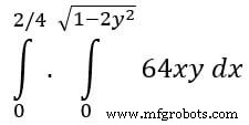
from scipy import integrate
import numpy as np
#import square root function from math lib
from math import sqrt
# set  fuction f(x)
f = lambda x, y : 64 *x*y
# lower limit of second integral
p = lambda x : 0
# upper limit of first integral
q = lambda y : sqrt(1 - 2*y**2)
# perform double integration
integration = integrate.dblquad(f , 0 , 2/4,  p, q)
print(integration)
출력:
(3.0, 9.657432734515774e-14)
위의 출력이 이전 출력과 동일한 것을 보았습니다.
| 패키지 이름 | 설명 |
|---|---|
| scipy.io |
|
| scipy.special |
|
| scipy.linalg |
|
| scipy.interpolate |
|
| scipy.optimize |
|
| scipy.stats |
|
| scipy.integrate |
|
| scipy.fftpack |
|
| scipy.signal |
|
| scipy.ndimage |
|
python
PyQt란 무엇입니까? PyQt 오픈 소스 위젯 툴킷 Qt의 파이썬 바인딩으로, 플랫폼 간 애플리케이션 개발 프레임워크로도 기능합니다. Qt는 모든 주요 데스크탑, 모바일 및 임베디드 플랫폼(Linux, Windows, MacOS, Android, iOS, Raspberry Pi 등 지원)용 GUI 애플리케이션을 작성하기 위한 인기 있는 C++ 프레임워크입니다. PyQt는 영국에 기반을 둔 회사인 Riverbank Computing에서 개발 및 유지 관리하는 무료 소프트웨어인 반면 Qt는 The Qt Company라는 핀란드 회
파이썬의 모듈은 무엇입니까? 모듈은 파이썬 코드가 있는 파일입니다. 코드는 정의된 변수, 함수 또는 클래스의 형태일 수 있습니다. 파일 이름이 모듈 이름이 됩니다. 예를 들어 파일 이름이 guru99.py이면 모듈 이름은 guru99가 됩니다. . 모듈 기능을 사용하면 한 파일 안에 모든 것을 작성하는 대신 코드를 여러 파일로 나눌 수 있습니다. 이 자습서에서는 다음을 배우게 됩니다. 파이썬의 모듈은 무엇입니까? 파이썬 가져오기 모듈 Python에서 모듈을 만들고 가져오는 방법은 무엇입니까? Python에서 클래스