산업 제조
산업용 사물 인터넷 | 산업자재 | 장비 유지 보수 및 수리 | 산업 프로그래밍 |
home  MfgRobots >> 산업 제조 >  >> Industrial materials >> 나노물질

나노안테나 입자 기반 지능형 약물 전달 시스템의 새로운 디자인

초록

복합 나노입자 약물 전달 시스템은 림프절과의 상호 작용에 중요한 역할을 합니다. 림프구에는 B 세포, T 세포 및 자연 살해 세포의 세 가지 기본 유형이 있습니다. 면역 체계의 세포가 발암성으로 바뀌면 신체 세포를 공격합니다. 림프액은 신체의 건강한 세포를 공격하는 데 중요한 역할을 합니다. 따라서 이 논문은 나노입자가 감염된 세포를 효율적으로 표적으로 하여 그러한 세포의 고속 제거를 도울 수 있는 약물 전달 시스템을 설계하는 것을 목표로 하고 있습니다. 제안된 디자인은 이러한 분자 간의 상호 작용에 따라 달라지며 지능형 나노 컨트롤러는 혐기성 접촉을 통해 나노 입자를 안내하는 기능을 가지고 있습니다. 제안된 디자인은 나노입자 크기와 밀도가 작을수록 액체의 동적 점도가 낮아서 흐름에 대한 저항을 반영한다는 것을 증명했습니다. 또한 수소 분자는 밀도가 낮아 림프액 저항을 줄이는 데 중요한 역할을 한다는 결론을 내렸습니다.

소개

현재 암 치료 옵션에는 수술, 방사선 및 화학 요법이 있습니다. 이러한 치료 전략은 또한 일반 조직에 해를 입히고 악성 성장을 부분적으로 소멸시킵니다. 따라서 나노기술은 유해한 세포와 ​​신생물을 구체적으로 표적화하고, 종양을 직접 절제하고, 방사선 기반 및 기타 치료 양식의 효과를 높임으로써 이러한 단점을 극복할 수 있습니다. 이것은 치료의 부작용을 크게 줄이고 생존율을 높일 수 있습니다. 나노 기술은 나노 물질을 사용하여 더 새롭고 더 나은 치료 양식을 제공하기 때문에 악성 성장 치료를 위한 유망한 도구입니다. 나노 입자는 암세포에서 차별적으로 발현되는 많은 분자를 특이적으로 표적화할 수 있습니다. 일반적으로 나노입자의 광대한 에어포일 영역은 작은 입자 및 디옥시리보핵 부식성 또는 리보핵 부식성 사슬 펩티드 항체와 같은 리간드로 기능화될 수 있습니다. 리간드는 약물 및 치료학 응용 분야에서 사용됩니다. 활력 산만 및 재방사선과 같은 나노 입자의 물리적 특성은 레이저 제거 및 온열 요법과 같이 병든 조직에 영향을 미치는 데에도 사용될 수 있습니다[1].

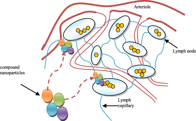
혁신적인 나노입자 소프트웨어 프로그램과 활성 제약 요소는 활성 성분의 더 넓은 레퍼토리를 탐색할 수도 있습니다. 따라서 면역원성 카고 및 표면 코트는 나노입자 매개 및 전통적인 화학요법에 대한 보조제로 조사되고 있습니다. 이 혁신적인 전략에는 항종양 효과를 발휘하는 자극 인자의 생체 내 저장소 및 세포에 제시하는 인공 항원으로서 나노입자의 설계가 포함됩니다. 나노 기술은 많은 응용 분야에서 활발한 연구 영역을 나타냅니다. 나노 입자는 해동 지수점, 친수성, 전기 및 열 전도, 촉매 활성, 광 흡수 및 산란과 같은 조정 가능한 물리 화학적 특성으로 인해 의료 기술에 관심을 갖게 되었습니다[2]. 원칙적으로 나노물질은 1~100 nm 범위의 입자를 가진 물질로 설명됩니다. 유럽 ​​연합과 미국에는 나노 물질을 사용한 의학 연구와 관련하여 몇 가지 법률이 있습니다. 그러나 국제적으로 통용되는 나노물질에 대한 정의는 없습니다. 다른 조직은 나노물질의 다른 개념을 고려합니다[3]. 나노입자 약물 전달 시스템의 목적 중 하나는 암세포로 림프액을 치료하는 것입니다. 림프절과 상호작용하는 복합 나노입자 약물 전달 시스템은 그림 1에 나와 있습니다.

<그림>

복합 나노입자 약물 전달 시스템 및 림프절과의 상호 작용

미국 식품의약국(FDA)은 나노물질을 벌크 물질과 특성이 다른 1~100개 범위의 입자를 갖는 물질로 언급하고 있다[4, 5]. 나노섬유, 나노플레이트, 나노와이어, 양자점 및 기타 관련 재료가 특성화되었습니다[6]. 고체 지질 나노입자(SLN)는 지질 나노입자(LN)의 일종으로 고체 지질을 활용하여 구성할 수 있습니다[7]. LN의 두 번째 시대를 나타내는 NLC(nanostructured lipid carriers)와 같은 SLN의 후속 버전이 개발되었습니다[8]. SLN과 NLC는 모두 고체 지질로 만들어집니다. SLN의 내부 구조는 고체 지질을 포함하는 반면 NLC는 보석 단면을 생성하는 고체 및 액체 지질의 혼합물을 사용하여 개발됩니다[9, 10]. 이러한 결함은 많은 고체 지질 세그먼트를 포함하는 SLN이 의료 응용 분야에서 사용될 수 있다는 사실에 비추어 SLN에 대해 추가로 보고되었습니다[11, 12]. 고분자 나노입자(PN)는 천연 고분자나 무기 재료(예:실리카)로 만들 수 있습니다[13]. 폴리머 또는 지질은 NP의 핵심을 형성하여 안정성과 약물 전달을 개선하고 균일한 모양과 크기를 제공합니다[14]. PN은 나노캡슐 또는 나노구로 설명할 수 있습니다. 나노캡슐은 약물과 함께 소포 구조에 오일을 포함하고[15, 16], 나노구는 오일이 없는 고분자 사슬을 포함합니다[17, 18]. 약물은 폴리머와의 블렌딩을 통해 PN에 패킹됩니다. 약물의 혼입은 중합 시 나노입자에 보장됩니다. PN은 고분자 네트워크의 구성 요소에 약물을 용해, 산란 또는 인공적으로 흡착하여 로드됩니다[19, 20]. 림프구에는 B 세포, T 세포 및 자연 살해 세포의 세 가지 유형이 있습니다. B 세포는 침입하는 미생물을 공격하는 항체를 만드는 동시에 발암성이 되면 면역 체계도 공격합니다. 따라서 자가면역에서 림프액의 중요한 역할을 고려하여, 본 논문의 목적은 나노안테나 입자를 기반으로 하는 지능형 약물 전달 시스템을 설계하는 것이었다. 따라서 시스템은 다양한 양의 많은 나노 입자를 포함합니다. 다음 섹션에서는 지능형 약물 전달 시스템의 설계를 제시합니다.

나노 지능형 약물 전달 시스템 설계

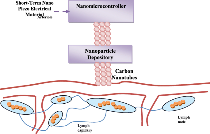
제안된 나노 지능형 약물 전달 시스템은 나노 압전 물질로 만들어진 나노 입자의 전원에 의해 작동되는 나노 컨트롤러를 포함합니다. 나노 입자의 복잡한 저장소에는 많은 마이크로 저장소가 있습니다. 각 작은 저장소에는 한 가지 유형의 나노 입자가 포함되어 있습니다. 나노 입자 분자는 나노 컨트롤러와 통신하도록 설계된 나노 안테나를 포함합니다. 제안된 나노 지능형 약물 전달 시스템은 또한 암세포에 약물을 신속하게 전달하기 위한 탄소 나노튜브를 포함합니다. 그림 2와 같이 감염된 세포와 연관될 수 있습니다. 시스템은 "탐색 나노입자"라고 불리는 암세포에 나노입자를 보내는 것으로 시작합니다. 이 분자들은 혐기성 통신을 통해 세포 내부의 위치에 대한 완전한 그림을 나노 컨트롤러에 보냅니다. 탐색적 나노입자가 직면한 상황에 따라 나노 컨트롤러는 탐색적 나노입자에서 수집된 정보를 기반으로 다양한 수, 유형 및 밀도의 나노입자를 암세포에 보냅니다. 이러한 나노입자를 "파이팅 나노입자"라고 합니다.

<그림>

감염된 세포와 제안된 약물 시스템의 연관성을 보여주는 일반 구조

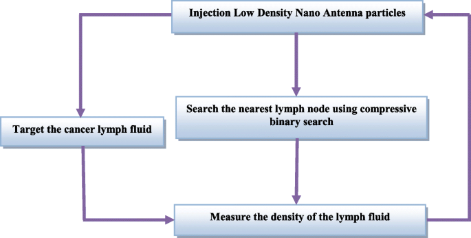
이것은 무작위 프로세스가 아니라 여러 측면과 로그를 고려하여 나노 컨트롤러에 의해 제어되어 나노 입자의 효율적이고 빠른 전달을 보장합니다. 나노입자를 암세포에 정확하고 빠르게 전달하기 위해 압축 이진 탐색 알고리즘이 사용될 것이다[21]. 또한 나노 입자는 다른 밀도로 전달되어 약물이 더 효과적입니다. 이러한 방법론과 나노컨트롤러를 이용한 작동방식은 그림 3과 같다. 나노컨트롤러의 물리적 구조는 나노입자와 유사하나 금속형태로 되어 있어 전기에너지를 얻을 수 있다. 일하는 동안 짧은 시간 동안. 이 금속에는 나노 컨트롤러와 나노입자 저장소 사이에 나노입자 링크가 있는 작동 코드가 포함된 작은 메모리와 함께 무선 안테나가 포함되어 있습니다. 나노 입자 저장소에는 여러 유형의 나노 입자가 포함되어 있습니다. 나노 게이트의 개폐 시간은 물론이고, 전달되는 입자의 수에 맞춰 조절될 것입니다.

<그림>

싸우는 나노입자를 암세포로 보내는 과정

제안된 약물 시스템에 사용되는 나노입자의 특성에 대한 설명

다음 섹션에서는 제안된 약물 전달 시스템에 사용된 나노입자의 특성에 대해 논의합니다. 이 연구에서 저밀도 혐기성 나노입자는 이전 보고서에서 설명한 대로 사용되었습니다[22].

저밀도 나노입자

종양이 림프액으로 둘러싸여 있는 림프액의 침투 과정으로 암에 대한 복합 나노입자의 약물 전달 과정을 고려하십시오. 흑색종의 구성은 림프액과 유사합니다. 제안된 분석 모델은 세 가지 다른 유형의 나노입자로 구성된 나노튜브 시스템을 기반으로 합니다. 나노 입자는 고밀도 림프액에 배치됩니다. 구형 극좌표에서 고체 A의 특정 나노입자를 A로 정의할 수 있습니다. =(라, ϑa , φa), 여기서 ra는 고체 A의 나노입자에 대한 방사 좌표이고, ϑa 는 고체 A의 나노입자에 대한 천정 좌표이고, φa는 고체 A의 나노입자에 대한 방위각 좌표입니다. 고체 B의 해당 좌표는 B입니다. =(rb, ϑb, φb)이고, 솔리드 N의 해당 좌표는 N입니다. =(rn, ϑn, φn) 림프절에는 호지킨 림프종의 암세포에 의해 영향을 받는 압통과 부종이라는 두 가지 특성이 있음을 고려하십시오. 부드러운 속성 Tp를 가진 림프절은 Tp(N , ); 이것은 고체 N의 나노 입자의 유체와 관련된 Tp 값이 시간에 따라 변한다는 것을 의미합니다. 이제 부드러운 속성에서 복합 나노입자의 총 효과가 다음과 같이 정의된다고 가정해 보겠습니다.

$$ \mathrm{Tpt}=\mathrm{Tp}\ \left(A,t\right)+\mathrm{Tp}\ \left(B,t\right)+.\dots \dots \dots \dots + \mathrm{Tp}\ \left(N,t\right) $$ (1)

다음과 같이 정의될 수 있는 팽창된 속성에 대한 동일한 경우를 고려하십시오.

$$ \mathrm{Tst}=\mathrm{Ts}\ \left(A,t\right)+\mathrm{Ts}\ \left(B,t\right)+.\dots \dots \dots \dots + \mathrm{Ts}\ \left(N,t\right) $$ (2)

식에서. 1과 2에서 시간에 따른 두 속성의 변화율은 다음과 같이 결정할 수 있습니다.

$$ \frac{\partial \left(\mathrm{Tp}\left(A,t\right)\right)}{\partial t}+\frac{\partial \left(\mathrm{Tp}\left( B,t\right)\right)}{\partial t}+\dots \frac{\partial \left(\mathrm{Tp}\left(N,t\right)\right)}{\partial t}=\frac{\mathrm{\partial Tp}(t)}{\mathrm{\partial t}} $$ (3) $$ \frac{\partial \left(\mathrm{Ts}\left(A,t\ right)\right)}{\partial t}+\frac{\partial \left(\mathrm{Ts}\left(B,t\right)\right)}{\partial t}+\dots \frac{\ 부분 \left(\mathrm{Ts}\left(N,t\right)\right)}{\partial t}=\frac{\mathrm{\partial Ts}(t)}{\partial t} $$ ( 4)

고체 N의 나노입자 하나가 차지할 수 있는 림프액의 점은 다음과 같이 정의됩니다.

$$ {\mathrm{Po}}_n=\mathrm{Po}{\left(\mathrm{po},t\right)}_n $$ (5)

부드러운 림프액의 고체 N 유도체의 나노입자가 \( \frac{\partial {\left(\mathrm{Tp}\left(N,t\right)\right)}_{\ mathrm{po}}}{\partial t} \), 부드러운 림프액의 복합 물질 파생물은 다음과 같습니다.

$$ \frac{\partial {\left(\mathrm{Tp}\left(A,t\right)\right)}_{\mathrm{po}}}{\partial t}+\frac{\partial { \left(\mathrm{Tp}\left(B,t\right)\right)}_{\mathrm{po}}}{\partial t}+\dots \frac{\partial {\left(\mathrm{ Tp}\left(N,t\right)\right)}_{\mathrm{po}}}{\partial t}=\frac{\mathrm{\partial Tp}{(t)}_{\mathrm{ po}}}{\partial t} $$ (6) $$ \frac{\partial {\left(\mathrm{Ts}\left(A,t\right)\right)}_{\mathrm{po} }}{\partial t}+\frac{\partial {\left(\mathrm{Ts}\left(B,t\right)\right)}_{\mathrm{po}}}{\partial t}+ \dots \frac{\partial {\left(\mathrm{Ts}\left(N,t\right)\right)}_{\mathrm{po}}}{\partial t}=\frac{\mathrm{ \partial Ts}{(t)}_{\mathrm{po}}}{\partial t} $$ (7)

고체 N의 해당 속도 성분은 (v rn , v ϑn , v φn ). 그러면 고체 N 입자의 유속은 림프액의 동점도 dv, p에서 나비에-스토크스 방정식을 사용하여 표현됩니다. 는 압력 및 ρ 는 다음과 같은 림프액의 밀도입니다.

$$ \frac{\partial {v}_{\mathrm{rn}}}{\partial t}+{v}_{\mathrm{rn}}\frac{\partial {v}_{\mathrm{rn }}}{\mathrm{\partial rn}}+\frac{v_{\upvartheta \mathrm{n}}}{\mathrm{rn}}\frac{\partial {v}_{\mathrm{rn}} }{\mathrm{\partial \upvartheta n}}+\frac{v_{\upvarphi \mathrm{n}}}{\mathrm{rn}\ \mathrm{sin}\upvartheta \mathrm{n}}\frac{ \partial {v}_{\mathrm{rn}}}{\mathrm{\partial \upvarphi n}}-\frac{v_{\upvartheta \mathrm{n}}^2}{\mathrm{rn}}- \frac{v_{\upvarphi \mathrm{n}}^2}{\mathrm{rn}}+\frac{1}{\rho}\frac{\partial p}{\mathrm{\partial rn}}- \mathrm{d}\upnu \left[\frac{1}{{\mathrm{rn}}^2}\frac{\partial }{\mathrm{\partial rn}}\left({\mathrm{rn} }^2\frac{\partial {v}_{\mathrm{rn}}}{\mathrm{\partial rn}}\right)+\frac{1}{{\mathrm{rn}}^2\mathrm {sin}\upvartheta \mathrm{n}}\frac{\partial }{\mathrm{\partial \upvartheta n}}\left(\mathrm{sin}\upvartheta \mathrm{n}\frac{\partial {v }_{\mathrm{rn}}}{\mathrm{\partial \upvartheta n}}\right)+\frac{1}{{\mathrm{rn}}^2{\sin}^2\upvartheta \mathrm {n}}\frac{\partial^2{v}_{\ma thrm{rn}}}{\partial {\upvarphi \mathrm{n}}^2}+-\frac{2{v}_{\mathrm{rn}}}{{\mathrm{rn}}^2} -\frac{2}{{\mathrm{rn}}^2\sin \upvartheta \mathrm{n}}\frac{\partial \left({v}_{\upvartheta \mathrm{n}}\mathrm{ sin}\upvartheta \mathrm{n}\right)}{\mathrm{\partial \upvartheta n}}-\frac{2}{{\mathrm{rn}}^2\mathrm{sin}\upvartheta \mathrm{ n}}\frac{\partial {v}_{\upvarphi \mathrm{n}}}{\partial_{\upvarphi \mathrm{n}}}\right]=0 $$ (8)

림프액의 동적 점도 dv는 다음과 같이 계산됩니다.

$$ \mathrm{d}\upnu =\frac{\left[\frac{\partial {v}_{\mathrm{rn}}}{\partial t}+{v}_{\mathrm{rn}} \frac{\partial {v}_{\mathrm{rn}}}{\mathrm{\partial rn}}+\frac{v_{\upvartheta \mathrm{n}}\partial {v}_{\mathrm{ rn}}}{\mathrm{rn}\ \mathrm{\partial \upvartheta n}}+\frac{v_{\upvarphi \mathrm{n}}}{\mathrm{rn}\ \mathrm{sin}\upvartheta \mathrm{n}}\frac{\partial {v}_{\mathrm{rn}}}{\mathrm{\partial \upvarphi n}}-\frac{v_{\upvartheta \mathrm{n}}^2 }{\mathrm{rn}}-\frac{v_{\upvarphi \mathrm{n}}^2}{\mathrm{rn}}+\frac{1\ \partial p}{\uprho \partial \mathrm{ rn}}\right]}{\left[\frac{1}{{\mathrm{rn}}^2}\frac{\partial }{\mathrm{\partial rn}}\left({\mathrm{rn }}^2\frac{\partial {v}_{\mathrm{rn}}}{\mathrm{\partial rn}}\right)+\frac{1}{{\mathrm{rn}}^2\ mathrm{sin}\upvartheta \mathrm{n}}\frac{\partial }{\mathrm{\partial \upvartheta n}}\left(\mathrm{sin}\upvartheta \mathrm{n}\frac{\partial { v}_{\mathrm{rn}}}{\mathrm{\partial \upvartheta n}}\right)+\frac{1}{{\mathrm{rn}}^2{\sin}^2\upvartheta \ 수학{n}}\frac{\partial ^2{v}_{\mathrm{rn}}}{\partial {\upvarphi \mathrm{n}}^2}+-\frac{2{v}_{\mathrm{rn}}}{{\ mathrm{rn}}^2}-\frac{2}{{\mathrm{rn}}^2\sin \upvartheta \mathrm{n}}\frac{\partial \left({v}_{\upvartheta \ mathrm{n}}\mathrm{sin}\upvartheta \mathrm{n}\right)}{\mathrm{\partial \upvartheta n}}-\frac{2}{{\mathrm{rn}}^2\mathrm {sin}\upvartheta \mathrm{n}}\frac{\partial {v}_{\upvarphi \mathrm{n}}}{\partial_{\upvarphi \mathrm{n}}}\right]} $$ ( 9)

고체 A와 B의 Navier-Stokes 방정식은 Eq로 나타낼 수 있습니다. 8 및 9. 따라서 Eq. 9는 다음과 같이 나타낼 수 있습니다.

$$ \mathrm{d}\upnu =\frac{\left[\frac{\partial {v}_{\mathrm{rn}}}{\partial t}+{v}_{\mathrm{rn}} \frac{\partial {v}_{\mathrm{rn}}}{\mathrm{\partial rn}}+\frac{v_{\upvartheta \mathrm{n}}}{\mathrm{rn}}\frac {\partial {v}_{\mathrm{rn}}}{\mathrm{\partial \upvartheta n}}+\frac{v_{\upvarphi \mathrm{n}}}{\mathrm{rn}\ \mathrm {죄}\upvartheta \mathrm{n}}\frac{\partial {v}_{\mathrm{rn}}}{\mathrm{\partial \upvarphi n}}-\frac{v_{\upvartheta \mathrm{ n}}^2}{\mathrm{rn}}-\frac{v_{\upvarphi \mathrm{n}}^2}{\mathrm{rn}}+\frac{1}{\rho}\frac{ \partial p}{\mathrm{\partial rn}}\right]}{\left[\frac{1}{{\mathrm{rn}}^2}\frac{\partial }{\mathrm{\partial rn }}\left({\mathrm{rn}}^2\frac{\partial {v}_{\mathrm{rn}}}{\mathrm{\partial rn}}\right)+\frac{1}{ {\mathrm{rn}}^2\mathrm{sin}\upvartheta \mathrm{n}}\frac{\partial }{\mathrm{\partial \upvartheta n}}\left(\mathrm{sin}\upvartheta \ mathrm{n}\frac{\partial {\mathrm{v}}_{\mathrm{rn}}}{\mathrm{\partial \upvartheta n}}\right)+\frac{1}{{\mathrm{ rn}}^2{\sin}^2\upvartheta \math rm{n}}\frac{\partial^2{\mathrm{v}}_{\mathrm{rn}}}{\partial {\upvarphi \mathrm{n}}^2}-\frac{2{\ mathrm{v}}_{\mathrm{rn}}}{{\mathrm{rn}}^2}-\frac{2}{{\mathrm{rn}}^2\sin \upvartheta \mathrm{n} }\frac{\partial \left({\mathrm{v}}_{\upvartheta \mathrm{n}}\mathrm{sin}\upvartheta \mathrm{n}\right)}{\mathrm{\partial \upvartheta n}}-\frac{2}{{\mathrm{rn}}^2\mathrm{sin}\upvartheta \mathrm{n}}\frac{\partial {\mathrm{v}}_{\upvarphi \mathrm {n}}}{\partial_{\upvarphi \mathrm{n}}}\right]}=\frac{\left[\frac{\partial {\mathrm{v}}_{\mathrm{ra}}} {\mathrm{\partial t}}+{\mathrm{v}}_{\mathrm{ra}}\frac{\partial {\mathrm{v}}_{\mathrm{ra}}}{\mathrm{ \partial ra}}+\frac{{\mathrm{v}}_{\upvartheta \mathrm{a}}}{\mathrm{ra}}\frac{\partial {\mathrm{v}}_{\mathrm {ra}}}{\mathrm{\partial \upvartheta a}}+\frac{{\mathrm{v}}_{\upvarphi \mathrm{a}}}{\mathrm{ra}\ \mathrm{sin} \upvartheta \mathrm{a}}\frac{\partial {\mathrm{v}}_{\mathrm{ra}}}{\mathrm{\partial \upvarphi a}}-\frac{{\mathrm{v} }_{\upvartheta \mathrm{a}}^2}{\mathrm{ra}}- \frac{{\mathrm{v}}_{\upvarphi \mathrm{a}}^2}{\mathrm{ra}}+\frac{1}{\uprho}\frac{\mathrm{\partial p} }{\mathrm{\partial ra}}\right]}{\left[\frac{1}{{\mathrm{ra}}^2}\frac{\partial }{\mathrm{\partial ra}}\ 왼쪽({\mathrm{ra}}^2\frac{\partial {v}_{\mathrm{ra}}}{\mathrm{\partial ra}}\right)+\frac{1}{{\mathrm {ra}}^2\mathrm{sin}\upvartheta \mathrm{a}}\frac{\partial }{\mathrm{\partial \upvartheta a}}\left(\mathrm{sin}\upvartheta \mathrm{a }\frac{\partial {v}_{\mathrm{ra}}}{\mathrm{\partial \upvartheta a}}\right)+\frac{1}{{\mathrm{ra}}^2{\ sin}^2\upvartheta \mathrm{a}}\frac{\partial^2{v}_{\mathrm{ra}}}{\partial {\upvarphi \mathrm{a}}^2}-\frac{ 2{v}_{\mathrm{ra}}}{{\mathrm{ra}}^2}-\frac{2}{{\mathrm{ra}}^2\sin \upvartheta \mathrm{a}} \frac{\partial \left({v}_{\upvartheta \mathrm{a}}\mathrm{sin}\upvartheta \mathrm{a}\right)}{\mathrm{\partial \upvartheta a}}-\ frac{2}{{\mathrm{ra}}^2\mathrm{sin}\upvartheta \mathrm{a}}\frac{\partial {v}_{\upvarphi \mathrm{a}}}{\partial_{ \upvarphi \mathrm{a}}}\right]}=\frac{ \left[\frac{\partial {v}_{\mathrm{rb}}}{\partial t}+{v}_{\mathrm{rb}}\frac{\partial {v}_{\mathrm{ rb}}}{\mathrm{\partial rb}}+\frac{v_{\upvartheta \mathrm{b}}}{\mathrm{rb}}\frac{\partial {v}_{\mathrm{rb} }}{\mathrm{\partial \upvartheta b}}+\frac{v_{\upvarphi \mathrm{b}}}{\mathrm{rb}\ \mathrm{sin}\upvartheta \mathrm{b}}\frac {\partial {v}_{\mathrm{rb}}}{\mathrm{\partial \upvarphi b}}-\frac{v_{\upvartheta \mathrm{b}}^2}{\mathrm{rb}} -\frac{v_{\upvarphi \mathrm{b}}^2}{\mathrm{rb}}+\frac{1}{\rho}\frac{\partial p}{\mathrm{\partial rb}} \right]}{\left[\frac{1}{{\mathrm{rb}}^2}\frac{\partial }{\mathrm{\partial rb}}\left({\mathrm{rb}}^ 2\frac{\partial {v}_{\mathrm{rb}}}{\mathrm{\partial rb}}\right)+\frac{1}{{\mathrm{rb}}^2\mathrm{sin }\upvartheta \mathrm{b}}\frac{\partial }{\mathrm{\partial \upvartheta b}}\left(\mathrm{sin}\upvartheta \mathrm{b}\frac{\partial {v}_ {\mathrm{rb}}}{\mathrm{\partial \upvartheta b}}\right)+\frac{1}{{\mathrm{rb}}^2{\sin}^2\upvartheta \mathrm{b }}\frac{\partial^2{v}_{\mathrm{ rb}}}{\partial {\upvarphi \mathrm{b}}^2}-\frac{2{v}_{\mathrm{rb}}}{{\mathrm{rb}}^2}-\frac {2}{{\mathrm{rb}}^2\sin \upvartheta \mathrm{b}}\frac{\partial \left({v}_{\upvartheta \mathrm{b}}\mathrm{sin}\ upvartheta \mathrm{b}\right)}{\mathrm{\partial \upvartheta b}}-\frac{2}{{\mathrm{rb}}^2\mathrm{sin}\upvartheta \mathrm{b}} \frac{\partial {v}_{\upvarphi \mathrm{b}}}{\partial_{\upvarphi \mathrm{b}}}\right]} $$ (10)

입자는 나노 차원입니다. 따라서 그들의 반지름은 매우 작을 것이고 간단하게 Eq. 10은 다음과 같이 표시됩니다.

$$ \mathrm{d}\upnu =\left[\frac{v_{\upvartheta \mathrm{n}}}{\mathrm{rn}}\frac{\partial {v}_{\mathrm{rn}} }{\mathrm{\partial \upvartheta n}}+\frac{v_{\upvarphi \mathrm{n}}}{\mathrm{rn}\ \mathrm{sin}\upvartheta \mathrm{n}}\frac{ \partial {v}_{\mathrm{rn}}}{\mathrm{\partial \upvarphi n}}-\frac{v_{\upvartheta \mathrm{n}}^2}{\mathrm{rn}}- \frac{v_{\upvarphi \mathrm{n}}^2}{\mathrm{rn}}+\frac{1}{\rho}\frac{\partial p}{\mathrm{\partial rn}}\ 오른쪽]/\left[\frac{1}{{\mathrm{rn}}^2}\frac{\partial }{\mathrm{\partial rn}}\left({\mathrm{rn}}^2\ frac{\partial {v}_{\mathrm{rn}}}{\mathrm{\partial rn}}\right)+\frac{1}{{\mathrm{rn}}^2\mathrm{sin}\ upvartheta \mathrm{n}}\frac{\partial }{\mathrm{\partial \upvartheta n}}\left(\mathrm{sin}\upvartheta \mathrm{n}\frac{\partial {\mathrm{v} }_{\mathrm{rn}}}{\mathrm{\partial \upvartheta n}}\right)+\frac{1}{{\mathrm{rn}}^2{\sin}^2\upvartheta \mathrm {n}}\frac{\partial^2{\mathrm{v}}_{\mathrm{rn}}}{\partial {\upvarphi \mathrm{n}}^2}-\frac{2{\mathrm {v}}_{\mathrm{rn}}}{{\math rm{rn}}^2}-\frac{2}{{\mathrm{rn}}^2\sin \upvartheta \mathm{n}}\frac{\partial \left({\mathrm{v}}_ {\upvartheta \mathrm{n}}\mathrm{sin}\upvartheta \mathrm{n}\right)}{\mathrm{\partial \upvartheta n}}-\frac{2}{{\mathrm{rn}} ^2\mathrm{sin}\upvartheta \mathrm{n}}\frac{\partial {\mathrm{v}}_{\upvarphi \mathrm{n}}}{\partial_{\upvarphi \mathrm{n}} }\right]=\left[\frac{{\mathrm{v}}_{\upvartheta \mathrm{a}}}{\mathrm{ra}}\frac{\partial {\mathrm{v}}_{ \mathrm{ra}}}{\mathrm{\partial \upvartheta a}}+\frac{{\mathrm{v}}_{\upvarphi \mathrm{a}}}{\mathrm{ra}\ \mathrm{ sin}\upvartheta \mathrm{a}}\frac{\partial {\mathrm{v}}_{\mathrm{ra}}}{\mathrm{\partial \upvarphi a}}-\frac{{\mathrm{ v}}_{\upvartheta \mathrm{a}}^2}{\mathrm{ra}}-\frac{{\mathrm{v}}_{\upvarphi \mathrm{a}}^2}{\mathrm {ra}}+\frac{1}{\uprho}\frac{\mathrm{\partial p}}{\mathrm{\partial ra}}\right]/\left[\frac{1}{{\mathrm {ra}}^2}\frac{\partial }{\mathrm{\partial ra}}\left({\mathrm{ra}}^2\frac{\partial {\mathrm{v}}_{\mathrm {ra}}}{\mathrm{\partial ra}}\rig ht)+\frac{1}{{\mathrm{ra}}^2\mathrm{sin}\upvartheta \mathrm{a}}\frac{\partial }{\mathrm{\partial \upvartheta a}}\left (\mathrm{sin}\upvartheta \mathrm{a}\frac{\partial {\mathrm{v}}_{\mathrm{ra}}}{\mathrm{\partial \upvartheta a}}\right)+\ frac{1}{{\mathrm{ra}}^2{\sin}^2\upvartheta \mathrm{a}}\frac{\partial^2{\mathrm{v}}_{\mathrm{ra}} }{\partial {\upvarphi \mathrm{a}}^2}-\frac{2{\mathrm{v}}_{\mathrm{ra}}}{{\mathrm{ra}}^2}-\ frac{2}{{\mathrm{ra}}^2\sin \upvartheta \mathrm{a}}\frac{\partial \left({\mathrm{v}}_{\upvartheta \mathrm{a}}\ mathrm{sin}\upvartheta \mathrm{a}\right)}{\mathrm{\partial \upvartheta a}}-\frac{2}{{\mathrm{ra}}^2\mathrm{sin}\upvartheta \ mathrm{a}}\frac{\partial {v}_{\upvarphi \mathrm{a}}}{\partial_{\upvarphi \mathrm{a}}}\right]=\left[\frac{v_{\ upvartheta \mathrm{b}}}{\mathrm{rb}}\frac{\partial {v}_{\mathrm{rb}}}{\mathrm{\partial \upvartheta b}}+\frac{v_{\ upvarphi \mathrm{b}}}{\mathrm{rb}\ \mathrm{sin}\upvartheta \mathrm{b}}\frac{\partial {v}_{\mathrm{rb}}}{\mathrm{\ 부분 \ upvarphi b}}-\frac{v_{\upvartheta \mathrm{b}}^2}{\mathrm{rb}}-\frac{v_{\upvarphi \mathrm{b}}^2}{\mathrm{rb }}+\frac{1}{\rho}\frac{\partial p}{\mathrm{\partial rb}}\right]/\left[\frac{1}{{\mathrm{rb}}^2 }\frac{\partial }{\mathrm{\partial rb}}\left({\mathrm{rb}}^2\frac{\partial {v}_{\mathrm{rb}}}{\mathrm{\ 부분 rb}}\right)+\frac{1}{{\mathrm{rb}}^2\mathrm{sin}\upvartheta \mathrm{b}}\frac{\partial }{\mathrm{\partial \upvartheta b}}\left(\mathrm{sin}\upvartheta \mathrm{b}\frac{\partial {v}_{\mathrm{rb}}}{\mathrm{\partial \upvartheta b}}\right)+ \frac{1}{{\mathrm{rb}}^2{\sin}^2\upvartheta \mathrm{b}}\frac{\partial^2{v}_{\mathrm{rb}}}{\ 부분 {\upvarphi \mathrm{b}}^2}-\frac{2{v}_{\mathrm{rb}}}{{\mathrm{rb}}^2}-\frac{2}{{\ mathrm{rb}}^2\sin \upvartheta \mathrm{b}}\frac{\partial \left({v}_{\upvartheta \mathrm{b}}\mathrm{sin}\upvartheta \mathrm{b} \right)}{\mathrm{\partial \upvartheta b}}-\frac{2}{{\mathrm{rb}}^2\mathrm{sin}\upvartheta \mathrm{b}}\frac{\partial { v}_{\upvarphi \mathrm{b}}}{\partial _{\upvarphi \mathrm{b}}}\right] $$ (11)

방정식 11은 다음과 같이 나타낼 수 있습니다.

$$ \mathrm{d}\upnu =\mathrm{rn}\left[{v}_{\upvartheta \mathrm{n}}\frac{\partial {v}_{\mathrm{rn}}}{\ mathrm{\partial \upvartheta n}}+\frac{v_{\upvarphi \mathrm{n}}}{\ \mathrm{sin}\upvartheta \mathrm{n}}\frac{\partial {v}_{\ mathrm{rn}}}{\mathrm{\partial \upvarphi n}}-{v}_{\upvartheta \mathrm{n}}^2-{v}_{\upvarphi \mathrm{n}}^2+ \frac{\mathrm{rn}}{\rho}\frac{\partial p}{\mathrm{\partial rn}}\right]/\left[\frac{\partial }{\mathrm{\partial rn} }\left({\mathrm{rn}}^2\frac{\partial {v}_{\mathrm{rn}}}{\mathrm{\partial rn}}\right)+\frac{1}{\ mathrm{sin}\upvartheta \mathrm{n}}\frac{\partial }{\mathrm{\partial \upvartheta n}}\left(\mathrm{sin}\upvartheta \mathrm{n}\frac{\partial { v}_{\mathrm{rn}}}{\mathrm{\partial \upvartheta n}}\right)+\frac{1}{\sin^2\upvartheta \mathrm{n}}\frac{\partial^ 2{v}_{\mathrm{rn}}}{\partial {\upvarphi \mathrm{n}}^2}-2{v}_{\mathrm{rn}}-\frac{2}{\sin \upvartheta \mathrm{n}}\frac{\partial \left({v}_{\upvartheta \mathrm{n}}\mathrm{sin}\upvartheta \mathrm{n}\right)}{\mathrm{\ 평가 tial \upvartheta n}}-\frac{2}{\mathrm{sin}\upvartheta \mathrm{n}}\frac{\partial {v}_{\upvarphi \mathrm{n}}}{\partial_{\ upvarphi \mathrm{n}}}\right]=\mathrm{ra}\left[{v}_{\upvartheta \mathrm{a}}\frac{\partial {v}_{\mathrm{ra}}} {\mathrm{\partial \upvartheta a}}+\frac{v_{\upvarphi \mathrm{a}}}{\ \mathrm{sin}\upvartheta \mathrm{a}}\frac{\partial {v}_ {\mathrm{ra}}}{\mathrm{\partial \upvarphi a}}-{v}_{\upvartheta \mathrm{a}}^2-{v}_{\upvarphi \mathrm{a}}^ 2+\frac{\mathrm{ra}}{\rho}\frac{\partial p}{\mathrm{\partial ra}}\right]/\left[\frac{\partial }{\mathrm{\partial ra}}\left({\mathrm{ra}}^2\frac{\partial {v}_{\mathrm{ra}}}{\mathrm{\partial ra}}\right)+\frac{1} {\mathrm{sin}\upvartheta \mathrm{a}}\frac{\partial }{\mathrm{\partial \upvartheta a}}\left(\mathrm{sin}\upvartheta \mathrm{a}\frac{\ 부분 {v}_{\mathrm{ra}}}{\mathrm{\partial \upvartheta a}}\right)+\frac{1}{\sin^2\upvartheta \mathrm{a}}\frac{\ 부분^2{v}_{\mathrm{ra}}}{\partial {\upvarphi \mathrm{a}}^2}-2{v}_{\mathrm{ra}}-\frac{2}{ \죄 \upvartheta \mathrm{a}}\frac{\partial \left({v}_{\upvartheta \mathrm{a}}\mathrm{sin}\upvartheta \mathrm{a}\right)}{\mathrm{\ 부분 \upvartheta a}}-\frac{2}{\mathrm{sin}\upvartheta \mathrm{a}}\frac{\partial {v}_{\upvarphi \mathrm{a}}}{\partial_{\ upvarphi \mathrm{a}}}\right]=\mathrm{rb}\left[{v}_{\upvartheta \mathrm{b}}\frac{\partial {v}_{\mathrm{rb}}} {\mathrm{\partial \upvartheta b}}+\frac{v_{\upvarphi \mathrm{b}}}{\ \mathrm{sin}\upvartheta \mathrm{b}}\frac{\partial {v}_ {\mathrm{rb}}}{\mathrm{\partial \upvarphi b}}-{v}_{\upvartheta \mathrm{b}}^2-{v}_{\upvarphi \mathrm{b}}^ 2+\frac{\mathrm{rb}}{\rho}\frac{\partial p}{\mathrm{\partial rb}}\right]/\left[\frac{\partial }{\mathrm{\partial rb}}\left({\mathrm{rb}}^2\frac{\partial {v}_{\mathrm{rb}}}{\mathrm{\partial rb}}\right)+\frac{1} {\mathrm{sin}\upvartheta \mathrm{b}}\frac{\partial }{\mathrm{\partial \upvartheta b}}\left(\mathrm{sin}\upvartheta \mathrm{b}\frac{\ 부분 {v}_{\mathrm{rb}}}{\mathrm{\partial \upvartheta b}}\right)+\frac{1}{\si n^2\upvartheta \mathrm{b}}\frac{\partial^2{v}_{\mathrm{rb}}}{\partial {\upvarphi \mathrm{b}}^2}-2{v} _{\mathrm{rb}}-\frac{2}{\sin \upvartheta \mathrm{b}}\frac{\partial \left({v}_{\upvartheta \mathrm{b}}\mathrm{sin }\upvartheta \mathrm{b}\right)}{\mathrm{\partial \upvartheta b}}-\frac{2}{\mathrm{sin}\upvartheta \mathrm{b}}\frac{\partial {v }_{\upvarphi \mathrm{b}}}{\partial_{\upvarphi \mathrm{b}}}\right] $$ (12)

나노 입자의 반경과 암으로 인한 림프 점도 사이에는 직접적인 관계가 있습니다. 림프가 너무 정체되고 점성이 있으면 순환하고 독소를 청소하고 암과 싸우는 데 도움이 되는 기능을 제대로 수행할 수 없습니다. 나노입자의 크기가 작으면 림프암 세포를 죽이기 쉽습니다. 화합물 나노입자의 총량의 이동을 설명하기 위해 연속 방정식을 사용하고 다음과 같이 고체 A, B 및 N의 세 가지 나노입자를 가정합니다.

$$ \frac{1}{{\mathrm{ra}}^2}\frac{\partial }{\mathrm{\partial ra}}\left({\mathrm{ra}}^2{v}_{ \mathrm{ra}}\right)+\frac{1}{\mathrm{ra}\ \mathrm{sin}\upvartheta \mathrm{a}}\frac{\partial }{\mathrm{\partial \upvartheta a }}\left(\sin {\upvartheta \mathrm{v}}_{\upvartheta \mathrm{a}}\right)+\frac{1}{\mathrm{ra}\ \mathrm{sin}\upvartheta \ mathrm{a}}\frac{\partial {v}_{\upvarphi \mathrm{a}}}{\mathrm{\partial \upvarphi a}}+\frac{1}{{\mathrm{rb}}^ 2}\frac{\partial }{\mathrm{\partial rb}}\left({\mathrm{rb}}^2{v}_{\mathrm{rb}}\right)+\frac{1}{ \mathrm{rb}\ \mathrm{sin}\upvartheta \mathrm{b}}\frac{\partial }{\mathrm{\partial \upvartheta b}}\left(\sin {\upvartheta v}_{\upvartheta \mathrm{b}}\right)+\frac{1}{\mathrm{rb}\ \mathrm{sin}\upvartheta \mathrm{b}}\frac{\partial {v}_{\upvarphi \mathrm{ b}}}{\mathrm{\partial \upvarphi b}}+\frac{1}{{\mathrm{rn}}^2}\frac{\partial }{\mathrm{\partial rn}}\left( {\mathrm{rn}}^2{v}_{\mathrm{rn}}\right)+\frac{1}{\mathrm{rn}\ \mathrm{sin}\upvartheta \mathrm{n}}\ frac{\parti 알 }{\mathrm{\partial \upvartheta n}}\left(\sin {\upvartheta v}_{\upvartheta \mathrm{n}}\right)+\frac{1}{\mathrm{rn}\ \ mathrm{sin}\upvartheta \mathrm{n}}\frac{\partial {v}_{\upvarphi \mathrm{n}}}{\mathrm{\partial \upvarphi n}}=0 $$ (13)

동적 유체 점도는 다음 방정식 [23]에서 결정할 수 있습니다.

$$ \mathrm{Vs}=\frac{2}{9}\frac{r^2g\ \left(\uprho \mathrm{p}-\uprho \mathrm{f}\right)}{\mathrm{dv }} $$ (14)

where Vs is the particles’ settling velocity (m/s), r is the Stokes radius of the particle (m), g is the gravitational acceleration (m/s 2 ), ρp is the density of the particles (kg/m 3 ), ρf is the density of the fluid (kg/m 3 ), and dv is the (dynamic) fluid viscosity (Pa·s). The lymph fluid is slightly heavier than water (lymph density = 1019 kg/m 3 , water density = 998.28 kg/m 3 at 20 °C). As a reference value, we consider the dynamic viscosity of the water to be 1.002 × 10 –3  kg m –1  s –1 ).

Dynamic viscosity is the measurement of the fluid’s internal resistance to flow, while kinematic viscosity refers to the ratio of dynamic viscosity to density. The effect of all the nanoparticles on the fluid viscosity is represented as follows:

$$ \mathrm{dv}=\frac{2\mathrm{g}}{9}\left[\frac{{\mathrm{ra}}^2\left(\uprho \mathrm{a}-\uprho \mathrm{f}\right)}{\mathrm{vsa}}+\frac{{\mathrm{rb}}^2\left(\uprho \mathrm{b}-\uprho \mathrm{f}\right)}{\mathrm{vsb}}+\frac{{\mathrm{rn}}^2\left(\uprho \mathrm{n}-\uprho \mathrm{f}\right)}{\mathrm{vn}}\right] $$ (15)

By comparing Eq. 12 and Eq. 15, the following equation could be emerged:

$$ \left|\frac{2\mathrm{g}}{9}\left[\frac{{\mathrm{ra}}^2\left(\uprho \mathrm{a}-\uprho \mathrm{f}\right)}{\mathrm{vsa}}+\frac{{\mathrm{rb}}^2\left(\uprho \mathrm{b}-\uprho \mathrm{f}\right)}{\mathrm{vsb}}+\frac{{\mathrm{rn}}^2\left(\uprho \mathrm{n}-\uprho \mathrm{f}\right)}{\mathrm{vn}}\right]\right|=\mathrm{rn}\left[{v}_{\upvartheta \mathrm{n}}\frac{\partial {v}_{\mathrm{rn}}}{\mathrm{\partial \upvartheta n}}+\frac{v_{\upvarphi \mathrm{n}}}{\ \mathrm{sin}\upvartheta \mathrm{n}}\frac{\partial {v}_{\mathrm{rn}}}{\mathrm{\partial \upvarphi n}}-{v}_{\upvartheta \mathrm{n}}^2-{v}_{\upvarphi \mathrm{n}}^2+\frac{\mathrm{rn}}{\uprho \mathrm{f}}\frac{\mathrm{\partial p}}{\mathrm{\partial rn}}\right]/\left[\frac{\partial }{\mathrm{\partial rn}}\left({\mathrm{rn}}^2\frac{\partial {v}_{\mathrm{rn}}}{\mathrm{\partial rn}}\right)+\frac{1}{\mathrm{sin}\upvartheta \mathrm{n}}\frac{\partial }{\mathrm{\partial \upvartheta n}}\left(\mathrm{sin}\upvartheta \mathrm{n}\frac{\partial {v}_{\mathrm{rn}}}{\mathrm{\partial \upvartheta n}}\right)+\frac{1}{\sin^2\upvartheta \mathrm{n}}\frac{\partial^2{v}_{\mathrm{rn}}}{\partial {\upvarphi \mathrm{n}}^2}-2{v}_{\mathrm{rn}}-\frac{2}{\sin \upvartheta \mathrm{n}}\frac{\partial \left({v}_{\upvartheta \mathrm{n}}\mathrm{sin}\upvartheta \mathrm{n}\right)}{\mathrm{\partial \upvartheta n}}-\frac{2}{\mathrm{sin}\upvartheta \mathrm{n}}\frac{\partial {v}_{\upvarphi \mathrm{n}}}{\partial_{\upvarphi \mathrm{n}}}\right]=\mathrm{ra}\left[{v}_{\upvartheta \mathrm{a}}\frac{\partial {v}_{\mathrm{ra}}}{\mathrm{\partial \upvartheta a}}+\frac{v_{\upvarphi \mathrm{a}}}{\ \mathrm{sin}\upvartheta \mathrm{a}}\frac{\partial {v}_{\mathrm{ra}}}{\mathrm{\partial \upvarphi a}}-{v}_{\upvartheta \mathrm{a}}^2-{v}_{\upvarphi \mathrm{a}}^2+\frac{\mathrm{ra}}{\uprho \mathrm{f}}\frac{\partial p}{\mathrm{\partial ra}}\right]/\left[\frac{\partial }{\mathrm{\partial ra}}\left({\mathrm{ra}}^2\frac{\partial {v}_{\mathrm{ra}}}{\mathrm{\partial ra}}\right)+\frac{1}{\mathrm{sin}\upvartheta \mathrm{a}}\frac{\partial }{\mathrm{\partial \upvartheta a}}\left(\mathrm{sin}\upvartheta \mathrm{a}\frac{\partial {v}_{\mathrm{ra}}}{\mathrm{\partial \upvartheta a}}\right)+\frac{1}{\sin^2\upvartheta \mathrm{a}}\frac{\partial^2{v}_{\mathrm{ra}}}{\partial {\upvarphi \mathrm{a}}^2}-2{v}_{\mathrm{ra}}-\frac{2}{\sin \upvartheta \mathrm{a}}\frac{\partial \left({v}_{\upvartheta \mathrm{a}}\mathrm{sin}\upvartheta \mathrm{a}\right)}{\mathrm{\partial \upvartheta a}}-\frac{2}{\mathrm{sin}\upvartheta \mathrm{a}}\frac{\partial {v}_{\upvarphi \mathrm{a}}}{\partial_{\upvarphi \mathrm{a}}}\right]=\mathrm{rb}\left[{v}_{\upvartheta \mathrm{b}}\frac{\partial {v}_{\mathrm{rb}}}{\mathrm{\partial \upvartheta b}}+\frac{v_{\upvarphi \mathrm{b}}}{\ \mathrm{sin}\upvartheta \mathrm{b}}\frac{\partial {v}_{\mathrm{rb}}}{\mathrm{\partial \upvarphi b}}-{v}_{\upvartheta \mathrm{b}}^2-{v}_{\upvarphi \mathrm{b}}^2+\frac{\mathrm{rb}}{\uprho \mathrm{f}}\frac{\partial p}{\mathrm{\partial rb}}\right]/\left[\frac{\partial }{\mathrm{\partial rb}}\left({\mathrm{rb}}^2\frac{\partial {v}_{\mathrm{rb}}}{\mathrm{\partial rb}}\right)+\frac{1}{\mathrm{sin}\upvartheta \mathrm{b}}\frac{\partial }{\mathrm{\partial \upvartheta b}}\left(\mathrm{sin}\upvartheta \mathrm{b}\frac{\partial {v}_{\mathrm{rb}}}{\mathrm{\partial \upvartheta b}}\right)+\frac{1}{\sin^2\upvartheta \mathrm{b}}\frac{\partial^2{v}_{\mathrm{rb}}}{\partial {\upvarphi \mathrm{b}}^2}-2{v}_{\mathrm{rb}}-\frac{2}{\sin \upvartheta \mathrm{b}}\frac{\partial \left({v}_{\upvartheta \mathrm{b}}\mathrm{sin}\upvartheta \mathrm{b}\right)}{\mathrm{\partial \upvartheta b}}-\frac{2}{\mathrm{sin}\upvartheta \mathrm{b}}\frac{\partial {v}_{\upvarphi \mathrm{b}}}{\partial_{\upvarphi \mathrm{b}}}\right] $$ (16)

Equation 16 depicts the relationship between the density of the lymph fluid, the density of the nanoparticles of the compound drug system, and the radius of the nanoparticles. There is a positive correlation between the density of the lymph fluid and the density of the nanoparticles. The smaller the density and radius of nanoparticles, the lesser the density of the fluid will be. As established earlier, the decrease in the density of the lymph fluid leads to its inability to reproduce and reduce the ferocity of the disease. It can, therefore, be concluded that the tumor can be cured by minimizing the size of nanoparticles. These particles can reach in the range of up to 0.1 nm (i.e., Angstrom or picometer range). The particles of this size can act as the nucleus of drug delivery in this drug system. Equation 16 shows that radii of the nanoparticles in the proposed drug system are related to the effectiveness of the delivery system. Much lower sized nanoparticles can reduce the density of lymph fluid and the spread of the disease.

Nanoparticles with Nanoantennas

This study used the nanoparticle described in an earlier report [22] as an emissary with a nano-microcontroller. In the system, the proposed transmission distance is very small and compatible with the composition of nanoparticles. Thus, the middle gap can be neglected in mid-distance and is symbolized by C d . Further, R X  are the real part and the imaginary part of the anaerobic impedance. After neglecting the load of the intercellular space between the nanoparticles and the nano-microcontroller, R X can be calculated as follows [22]:

$$ {R}_a=\frac{r_{a0}}{1+{C}_d{w}_a\left(2{x}_{a0}+{C}_d\left({r_{a0}}^2+{x_{a0}}^2\right){w}_a\right)} $$ (17) $$ {X}_a=\frac{x_0-{C}_d\left({r_{a0}}^2+{x_{a0}}^2\right){w}_a}{1+{C}_d{w}_a\left(2{x}_{a0}+{C}_d\left({r_{a0}}^2+{x_{a0}}^2\right){w}_a\right)} $$ (18)

Thus, the load resistance value of nanotubes can be predicted as in the following equation:

$$ {r}_l=\frac{g^2R}{g^2-2 gSX{\varepsilon}_L\omega +{S}^2\left({R}^2+{X}^2\right){\varepsilon_L}^2{\omega}^2} $$ (19)

여기서 ε  is the permittivity of the loading material, g is the size of the gap, and S is the effective cross-section area of the gap. In order to simplify the equation, the value of g 2 can be neglected as it is too low and the final equation can be rewritten as follows:

$$ {r}_l=\frac{g^2R}{-2 gSX{\varepsilon}_L\omega +{S}^2\left({R}^2+{X}^2\right){\varepsilon_L}^2{\omega}^2} $$ (20)

Then,

$$ {r}_l=\frac{g^2R}{S{\varepsilon}_L\omega \left(-2 gX+S\left({R}^2+{X}^2\right){\varepsilon}_L\omega \right)} $$ (21)

The optical nano-photo concept can be used as an effective tool for interpreting and predicting these effects to design and improve nanoscale parameters and increase the nano-sensitivity to serve better as a single molecular sensor. Nanoantenna may provide optimal performance in terms of sensitivity, efficiency, and bandwidth in the process. The next section presents the concept of searching the cancerous lymph nodes using compressive binary search algorithm.

Searching for the Target Lymphatic Nodes Using Compressive Binary Search

In order for nanoparticles to reach the cancerous cells in a fast and efficient manner, we applied compressive binary search by the nano-microcontroller. The guided nanoparticles follow a specific path to quickly reach the target. This movement is based on the information obtained from the “exploratory nanoparticles.” Assume that the target lymph node, Tf, has exactly one nonzero entry, where the location of the lymph node is unknown. The algorithm divides mt measurements into a total of St stages, where St refers to the stages of the lymph nodes. The measurements are more than one for all the stages of the lymph nodes, which is necessary for the algorithm to be executed until completion. Based on this measurement, the algorithm decides between going left or right, until the nanoparticles reach the target, the cancerous lymph node.

결과 및 토론

In order to analyze the proposed design, the nanoparticles were applied to the following five types of materials:silicone, lithium, lung, helium, and hydrogen. The materials were chosen because of their low density. The lung nanoparticles were samples from nano-sized lung nodules. They appear encircling with white shadows in a chest X-ray or computerized tomography scan taken from the lung of the person and required to be undamaged. The proposed idea is based on the analytical model, which indicates that the smaller the density of nanoparticles, the smaller the dynamic viscosity will be. This will result in a decrease in fluid viscosity. It is shown that the types of materials and the density of each particle will affect settling velocity of nanoparticles at entry into the lymphatic fluid and the density of the lymphatic fluid. We considered the following parameters:acceleration of gravity (g ) = 9.80665, particle diameter (d ) = 10 A, initial density of lymph fluid (ρf) = 998.28, and dynamic viscosity = 0.0010 kg m –1  s –1 [24]. These parameters were selected by the assumption that the viscosity of the lymphatic fluid is very similar to the viscosity of the water and the very small difference does not affect the results of the model. Figure 4 illustrates the density of nanoparticles for five selected materials for application in the proposed analytical model. Figure 5 shows the settling velocity for each particle. Figure 6 shows the effect of the settling velocity of nanoparticles on altering the lymphocyte density of cancer cells. The results shown in Fig. 6 show that the settling velocity of the particles carries a negative value. This indicates that the nanoparticle after entering in the lymphatic fluid rapidly moves in the opposite direction toward their entry into the lymphatic fluid. In general, any object that moves in the negative direction has a negative velocity. This movement of the particle leads to reduced viscosity of the lymphatic fluid.

Density of nanoparticles for the five selected materials

The settling velocity data for each particle

The effect of the settling velocity of nanoparticles on changing the lymphocyte density of cancer cells

Silicone nanoparticles showed the settling velocity of approximately − 2.87 × 10–15 m/s. This resulted in a decrease in viscosity of the lymphatic fluid to 987.72 kg/m 3 for the initial density 998.28 kg/m 3 . The density is continuously reduced to a point where hydrogen produces extremely spectacular results, i.e., the complete collapse of lymphatic fluid resistance. The density of the lymphatic fluid − 856.28 kg/m 3 with the negative sign indicated that there was no resistance from the lymphatic fluid to the flow of the nanoparticles, resulting in the complete collapse of the liquid fluid. Both the hydrogen and helium particles have a significant impact on the liquid viscosity due to the low density of the particles. Hence, it is important to use a drug system consisting of a group of nanoparticles for low-density materials. Figure 7 shows the relationship between the diameters of lung nanoparticles and the number of nanoparticles in one group. The figure shows that the higher the diameter of nanoparticles, the fewer their number in a group. This is clearly shown at the highest value of the nanoparticle diameter of 1000 nm, where the number of molecules in a group is 20 molecules. Figure 8 shows the relationship between the diameters of lithium nanoparticles and the number of nanoparticles in one group. This figure demonstrates the inverse relationship between the radius of nanoparticles and the number of molecules in a group where lithium particle diameters are significantly lower than the lung nanoparticles, where the number of nanoparticles in Fig. 7 is relatively low compared to the lithium particles as shown in Fig. 8. And the multicolor balls in both figures refer to different ranges of nanoparticle radii for each group, where each group contains a number of nanoparticles with different sizes. The best results can be obtained when hydrogen and helium particles are increased from other substances. A mixture of different materials should be used so that the properties of these substances can be used in the treatment process as well as to reduce viscosity. Figure 9 illustrates the different sets of materials proposed to have the mean highest density of both hydrogen and helium materials. Figure 10 shows the average mass of a nanoparticle in a group. It can be seen that the mass of both hydrogen and helium is the highest compared to the mass of particles of other substances. Figure 11 illustrates the relationship between the diameters of the nanoparticles and the width of its group or class. It is important to note that these results will open up a new area to reduce the resistance of the lymphatic fluid in tumors. This can be achieved using hydrogen nanoparticles of a size in the range of Angstrom. In addition to hydrogen nanoparticles, there may also exist a number of other substances in the same size. Figure 12 illustrates the standard deviation of a number of coefficients for both lung and lithium nanoparticles. These coefficients are limited to fractions of nanoparticles in a single group as well as their number in addition to the diameters of these nanoparticles. It is clear that the group fractions have the less value of the standard deviation. Hence, most of the fractions in the computational processes are around the mean of these values. Figure 13 shows the standard deviation of the mass for particles of silicones, lithium, lungs, helium, and hydrogen in one group. It is clear that the particles of the lung have the largest standard deviation and the lithium has the minimum value.

Group of nanoparticles in the lung cells and their number in one of the proposed groups

Group of nanoparticles in the lithium cells and their number in one of the proposed groups

Different sets of materials proposed to have the mean highest density of both hydrogen and helium materials

Average mass of a nanoparticle in a group

Diameters of the nanoparticles related to the group width

The standard deviation of lung and lithium nanoparticles coefficients

The standard deviation of the mass for particles of silicones, lithium, lungs, helium, and hydrogen in one group

방법

The aim of this study was to establish a nano-drug delivery system capable of delivering the drugs effectively to the cancer cells. The following methodology was used to deliver nanoparticles:

  1. i)

    Low-density nanoparticles

This study proposed the theoretical approach of nanoparticles as a low-density drug. This depends on the density and the settling velocity of the nanoparticles, as these nanoparticles can overcome the resistance of the lymphatic fluid.

  1. ii)

    Preparation of anaerobic nanoparticles

This study uses the idea of nanoparticles possessing an antenna through which a connection can be made between nanoparticles and nano-controller. The transmission distance was assumed to be too small to match the composition of nanoparticles and also to fit the actual distance between them.

  1. iii)

    Nano-controller design

Its function is to deliver the nanoparticle drug to cancer cells. Its role is to send signals to the nanoparticles and coordinate their actions and direct them to the lymphatic fluid of tumors.

  1. iv)

    Searching for the target lymphatic nodes

The lymphatic nodes are searched using compressive binary search algorithm. This algorithm is characterized by high-speed search, which makes nanoparticles more accessible to infected cells than the conventional methods. The primary supervisor behind the performance of the nanoparticles is the nano-controller. It directs nanoparticles to the infected cells by following this algorithm to ensure that an appropriate number of molecules are in proportional density to the lymphatic fluid.

결론

There have been various studies managing the treatment of malignant growth utilizing nanoparticles. The lymphatic liquid in tumors plays a substantial role in the obstruction of medication to the cancer cells. We developed an intelligent drug delivery system containing a consortium of nanoparticles. The proposed design demonstrates that small nanoparticles result in low density of the fluid. The results indicated that hydrogen particles are most efficient in reducing resistance toward lymphatic liquid owing to their smaller size. Furthermore, the design involves an anaerobic nano-controller that can determine the state and area of the particles. This technique conveys the medication to the infected cell more effectively.

데이터 및 자료의 가용성

The datasets supporting the results of this article are included within the article.

약어

LN:

지질 나노입자

NLC:

Nanostructured lipid carriers

PN:

Polymeric nanoparticles

SLN:

고체 지질 나노입자


나노물질

  1. 고장 방지 설계
  2. 향상된 약물 전달을 위한 나노섬유 및 필라멘트
  3. 생체적합성 FePO4 나노입자:약물 전달, RNA 안정화 및 기능적 활성
  4. 종양 치료를 위한 약물 전달 시스템으로서의 환경 반응성 금속-유기 프레임워크
  5. 암 응용을 위한 세포 기반 약물 전달
  6. Zebrafish:나노기술 매개 신경특이성 약물 전달을 위한 유망한 실시간 모델 시스템
  7. 흑색종의 표적 화학요법 치료를 위한 약물 전달체로서의 131I-추적된 PLGA-지질 나노입자
  8. 새로운 나노입자 강화 벌레 유사 미셀 시스템 연구
  9. 나노기술:생체 내 이미징 시스템에서 약물 전달 제어까지
  10. 다기능 GaN/Fe 나노입자로 내피 세포 표적화